

Whether you're at the helm of an early-stage startup campaigning for funding, or a well-established organization looking to stay competitive, understanding the lifetime value of your customers is an essential guide to how much you can spend on customer acquisition and support.
Unfortunately, the usual way of calculating this critical metric rests on a lot of assumptions about your business — assumptions that are not usually met in the real world. If you rely on the usual way, you're missing out: at the very least, you're overlooking key insights and a deeper understanding of your customers and, at worst, you're getting information that's simply wrong.
We want to spread the word about these limitations, and take the opportunity to highlight a statistical-model-based approach we prefer here at Strong Analytics. To do this, we'll contrast the two approaches on real data from a subscription-based company with which we recently worked. But the lessons we'll learn from looking at this specific company will be general ones that apply to any business— including yours.
LTV: The Conventional Way
Lifetime value seems simple enough at first: it's just how much revenue the "typical" customer will bring in over their lifetime. For a monthly-subscription service (which our example dataset comes from), you can think of this as the typical customer's monthly payments, spread over the typical customer's account-duration.
However, you can't actually calculate LTV in this way — by multiplying average monthly revenue-per-account by the average account-duration. That's because — unless you're engaging in a post-mortem of a failed venture — you have a large contingent of customers who are still members and thus still generating revenue. For any current customer, their current account duration is necessarily an under-estimate of their trueaccount duration. If you want the lifetime of a typical customer, you won't get an accurate picture by taking the average account-duration.
Fortunately, a conventional approach to calculating LTV gets around this problem by transforming our question about durations to a question about rates. If I run at a rate of 10 miles per hour, then you should expect to wait an average duration of six minutes for me to complete each mile. This is how LTV is conventionally calculated. We start with the churn rate — the percentage of customers who cancel within a month — and take its reciprocal. This gives us the average account-duration (the average amount of time we expect to wait for a customer to cancel), which we then multiply by the average revenue per-customer per-month.
LTV = AverageRevenuePerAccount(ARPA) * ChurnRateLTV = AverageRevenuePerAccount(ARPA) * ChurnRate
Where an estimate of churn-rate might be:
ChurnRate = CustomersChurnedthisMonthTotalNum * CustomersLastMonthChurnRate = CustomersChurnedthisMonthTotalNum * CustomersLastMonth
Let's do these calculations for the dataset from our example company.
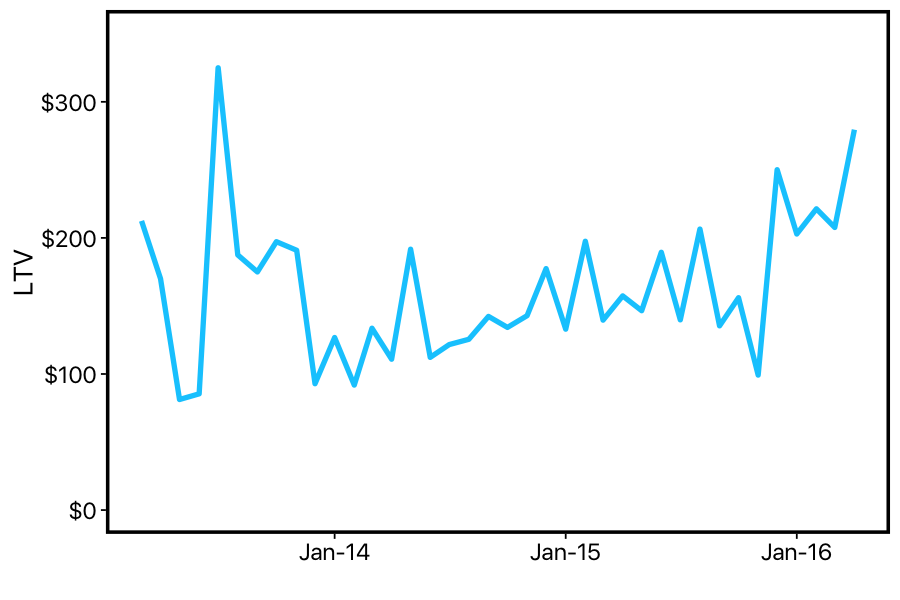
We can see that this estimate of LTV is extremely noisy: it varies a lot from month-to-month. But even through this noise, we can see that LTV is going up over time: since the company was founded, the general trend seems to be that customers are paying more and/or churning more slowly. Either way — good news, right? Time to update the pitch-decks for investors?
Not so fast. It may not seem like it from the simple formula above, but we've just made our first statistical model of the customer lifecycle. Like any model, it makes assumptions about the data that goes into it — which means assumptions about how the business operates and how the customers behave. The main assumption made here is that the 'churn rate' is constant over a customer's lifetime. In other words, the LTV calculation we just made is only valid if a customer has the same probability of cancelling their account no matter how long they've been with your company. This assumption can easily be wrong. Maybe lots of customers sign up initially, but are only really interested in using the product once and so quickly churn; while customers who have stuck around for a year are the type of people who use the product repeatedly and are unlikely to churn. Or things could be reversed: perhaps almost all customers feel like they get something useful out of the product in the first year, but after that they generally find that they've exhausted its usefulness.
You probably don't want to make critical decisions about your business based on faulty assumptions. If we're going to use a statistical model anyways, we might as well take a closer look at these assumptions, and figure out the right statistical model.
Finding the Right Statistical Model: Survival Analysis
So far we've used a simple formula for LTV. A more statistical description of this simple formula is that it assumes customers' account-durations are drawn from an exponential distribution. This distribution is meant to model waiting-times for events that have a constant probability of occurring. This distribution has a rate parameter, which we can think of as the probability of that event occurring in a given time-unit (e.g., a churn-rate is the probability of a customer cancelling each month).
Of course, many events don't occur at a constant rate. I might average a rate of 10 miles per hour... for the first 30 seconds of my run. After that, my rate quickly drops off — so you definitely shouldn't expect to wait 6 minutes for me to complete a mile. Events which don't have a constant probability of occurring over time can be modeled as coming from a weibull distribution. The Weibull distribution is a generalization of the exponential distribution, in which an extra parameter determines whether (and how quickly) the probability of the event increases or decreases over time.
Using a Weibull model of customer-lifetime frees us from the restrictive assumption that customers are equally likely to cancel throughout their lifetime. But it also means we can't do the quick-and-easy calculation we did before. Instead, in order to construct our model of customer lifetime, we'll recruit tools from an area of statistics known as "survival analysis."
"Survival analysis" deals with 'time-to-event' data, where the event of interest hasn't necessarily happened for everyone in our dataset. In our case, the 'event' is a customer cancelling their account. In survival analysis, we are interested in the 'survival' curve, which gives us a new way of expressing churn over time. Imagine all of your customers started at the exact same time, and you have a 15% churn rate. In the first month, you should expect (1 - .15) = 85% of the customers to be retained. In the second month, you should expect (1 - .15)*(1 - .15) = 72% of the original customers to be retained. In the third month, (1 - .15)^3 = 61%, etc.
This describes the process that might generate a survival curve, but we can also do things in the other direction: we can take all of customers' account durations, and plot the percentage of customers whose accounts are at least X number of months. Here's what that looks like for our dataset.
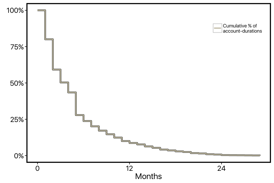
However, this curve isn't quite right yet: we aren't correctly factoring in customer who are still members. For example, there's a steep drop-off in the curve at 5-months, but this isn't because lots of customers cancelled at this point. There was just a big cohort of customers who started 5-months ago who are still members. In survival analysis, this is known as the problem of "censoring". The account-durations of the current customers are censored: we know that they are at least 5-months long, but we don't know how much longer than that they will ultimately be.
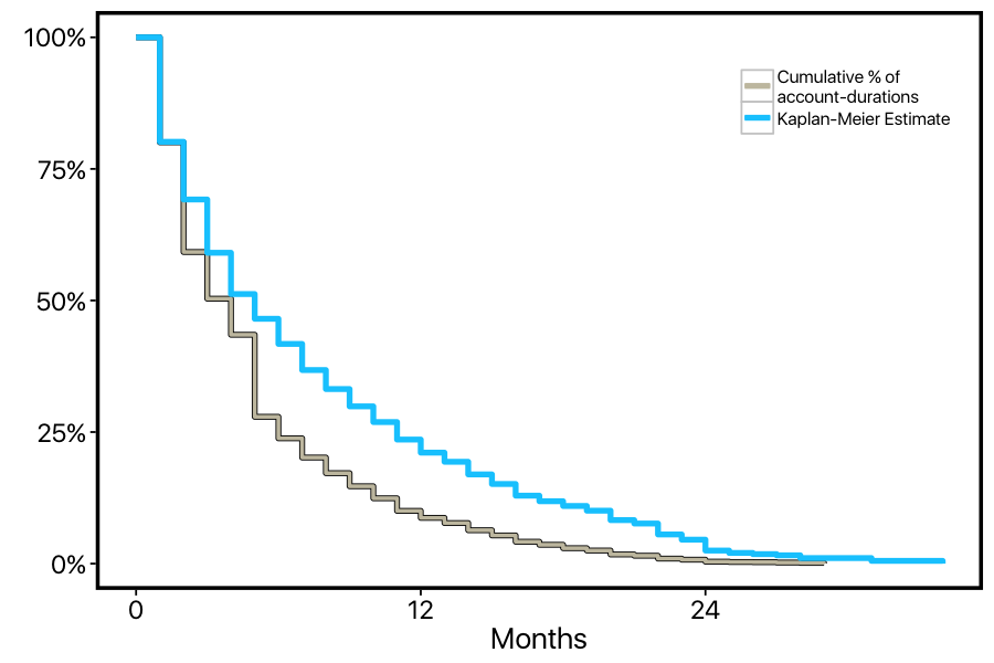
We can re-do our calculation of the curve in a way that correctly factors in these current customers. For customers who cancel, we'll lower the height of the curve just as before; but for customers who are "censored", we'll use them in the percentage calculations before they become censored, then simply remove them from these calculations at the point on the x-axis where they become censored. The resulting curve is called a "Kaplan-Meier" survival curve. We can see that this KM curve doesn't have the steep dropoff point at 5-months, and it's generally higher than the first curve, reflecting the fact that the original curve was under-estimating retention.
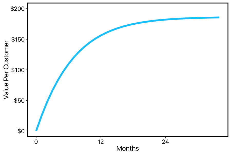
Now we have an estimate of how customers churn over time, one that correctly factors in 'censored' customers. We can finally fit our Weibull model to this data. Here we plot the inverse cumulative distribution function of a Weibull distribution fit to this data (using R's flexsurv package).
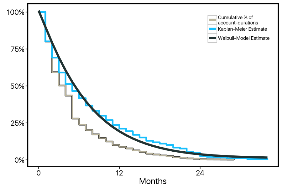
Our current model tells us that the 'shape' parameter of the weibull distribution is 1.08, with a 95% confidence interval of (1.05, 1.12). When this shape parameter is greater than one, it means the probability of the event increases over time (while shape < 1 means it decreases over time, and shape = 1 is just the exponential distribution). So our model suggests that the data we're looking at significantly deviates from the exponential-distribution model of constant churn over time: instead, the customers at this company become more likely to cancel the longer they remain subscribed.
LTV and Beyond with Survival Models
Now that we've got our survival model of customer lifetime, how can we use it to estimate lifetime value? A simple yet valuable property of the inverted cumulative distribution function we plotted above is that the area under this curve is the expected value — in our case, the average customer lifetime. (This might seem a little opaque, but it actually follows straightforwardly from how we made the curve. The average account-duration is just each account-duration multiplied by the proportion of times that account-duration occurs in the dataset. In the survival curve, if a customer has been around for 1-month, then they will take up one unit of area in the survival curve; if they've been around for 5-months, they will take up five units. Since each unit of area represents a proportion, we have account-duration times proportion — or the average account-duration.)
The nice thing about fitting a parametric model to our data is that — thanks to the wonders of calculus — we can calculate the area under our curve out to infinity. If we multiply this by the average price-per-month, we get an estimate of lifetime value. In this case, we get $186.
So far I've talked a lot about the statistics behind this new approach to estimating LTV. It's time to make this a bit more concrete and intuitive. While the quick-and-easy LTV calculation we started with gave us a measure that bounced around a lot from month-to-month, overall that measure doesn't seem to be too far off from the number we got from survival analysis. Was it worth all the extra work?
Advantage # 1: Better Estimates
Let's make things more concrete and consequential: let's imagine that exactly one year ago, our company started calculating LTV both ways: recording the back-of-the-envelope measure that assumes constant churn, and also recording the results of a Weibull survival-model. Now after a year of this experiment, we want to know which method was better.
How can we do this? One advantage to framing customer retention in terms of survival curves is that these curves don't just give us a single number. If we take the area under the curve between zero and infinity (and multiply it by average revenue), we'll get the LTV assuming our business keeps running indefinitely. But if we take the area under the curve between zero and twelve-months (again, times revenue), we'll get the expected revenue after one year. So our survival-curve can be used as a function that takes an amount of time we're willing to wait, and returns the expected revenue after waiting that long:
So after a year of calculating LTV two different ways, we want to compare our weibull model of customer lifetime to the conventional constant-churn-rate model. This should be easy enough: let's just look at all the customers who had active memberships one year ago when we started our experiment, and plug them into the graph above. This should tell us how much more money we should expect from each customer, based on how long they've been around. If we add this up, this estimate should be a number that's very close to how much revenue they actually brought it.
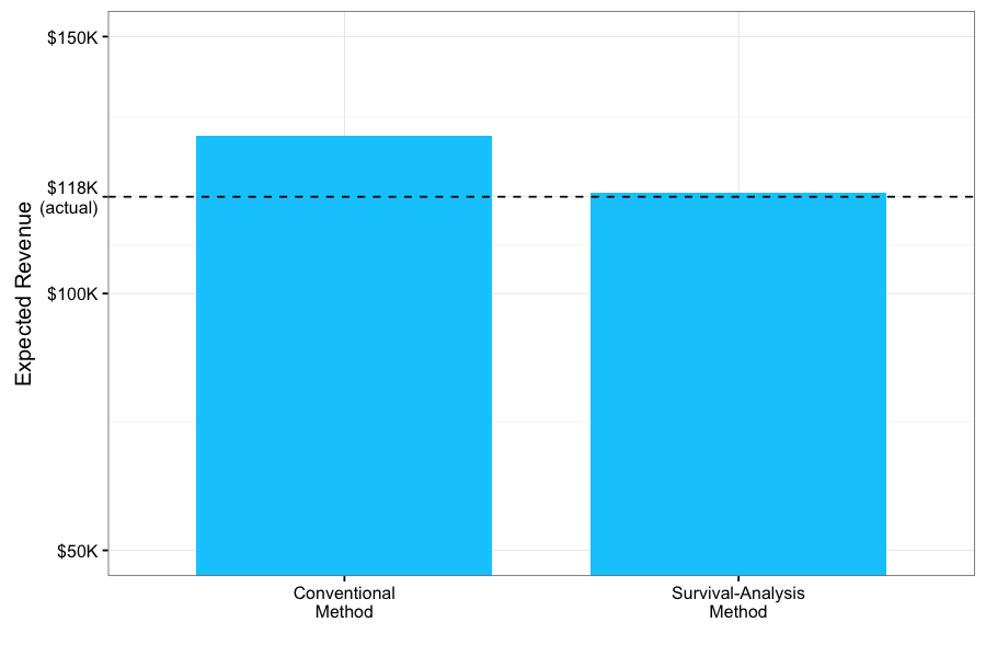
The results are clear. The conventional calculation applies the same churn-rate to all customers, regardless of their stage in their life-cycle. By optimistically assuming late-stage customers have the same probability of cancelling as early-stage ones, it over-estimates the revenue it expects to get from these late customers — leading to an overall over-estimate of almost twelve-thousand-dollars. In contrast, our Weibull model takes into consideration the life-cycle-stage of each customer in order to estimate how much more time (and value) we should expect from their membership on an individual basis.
Advantage # 2: Deeper insights about the Lifecycle
Another advantage to taking the survival-analysis approach is that it lets us investigate patterns in the customer life-cycle that aren't necessarily reflected in overall lifetime value.
One example of this is how customer-lifecycle has changed since the business featured here was originally founded. When we plotted our initial quick-and-easy LTV calculations, it looked like LTV was very slightly increasing over time. While this might have seemed like an indicator of business health, we now know that we can't necessarily trust this: if the business is constantly adding more and more customers, then this will artificially lower the churn rate (since, as we now know, new customers churn less than old customers). This shouldn't be confused with an increasing lifetime value among current customers.
Instead, we can examine how the survival curve of our customers has changed over the years. For now we can just pick an arbitrary split-point and compare:
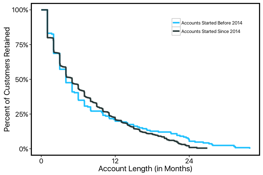
We can see from these curves that the customer lifecycle has been shifting over the years — even though the average account-duration hasn't actually changed! Customers have become more likely to stay in the early stages of their membership, but have become less persistently loyal in later stages of their membership. This is an important insight about a potentially shifting customer-base, with core bedrock customers becoming harder to come-by. This particular company has a social component to its services, with forums and community providing value to customers (more on that later). So a lack of bedrock loyal customers who help build the community might signal trouble for the company's future growth.
Advantage # 3: Customer-Segmentation and LTV
Above we got a glimpse into the advantages of segmenting our customer-base, splitting our survival curve by early vs. late adopters. We can extend this to a more general approach by incorporating covariates into our survival regression.
We implemented a Bayesian MCMC survival model (using the JAGS language) to estimate the effects of several predictors on customers' retention. In this framework, regression coefficients can affect both the 'shape' and 'scale' parameters of the weibull distribution, which can then be translated into effects on the survival curve and on LTV. For example, this company leaves it up to the customer whether they want to fill in extra profile information, such as their interests, website, and occupation. We can use this to split our customer-base into two groups, and plot the two KM-curves model estimates separately.
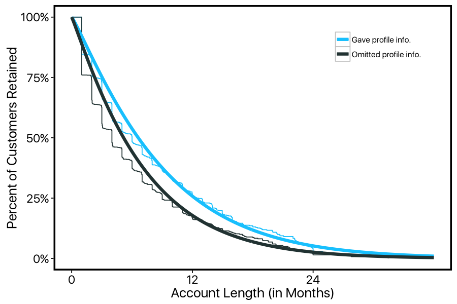
We can see that customers who fill in this optional profile information tend to stick around much longer on average, with their survival curve consistently above those who omit this profile info.
We can summarize the effect of predictors like this one on customers' LTV. For example, another predictor — whether or not a customer used the company's forums — had an average of $47 more lifetime value for every post they made per month! This is a dramatic effect.
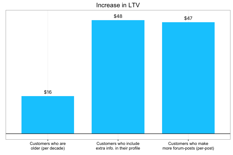
Estimating the effects of customer-attributes and behavior on their life-cycle can provide insights into what makes customers stay with your company, which in turn can provide valuable strategic guidance. For the company featured here, the large effect of forum activity suggests that the community-driven aspects of this company might be especially important to customers. This in turn suggests that promoting community-engagement could promote retention. Future directions would involve pursuing A/B testing to confirm this possibility.
Another reason that predicting LTV based on attributes of your customers can be valuable is that it tells you not just what affects LTV, but by how much. Especially if your company is in its early-stages, it's tempting to compute a single LTV number and assume this will remain stable as your company grows. In reality, as you acquire customers from new and diverse sources, LTV can change in ways you won't be ready for if you're just computing a single number. By understanding how segments of customers differ in their LTV, you can be better prepared for how your LTV will change as the composition of your customer-base changes. This kind of information can be valuable in knowing how much to spend on new acquisition or marketing strategies— from large-scale advertising campaigns to simple promotions for new customers.
Advantage # 4: Live Predictions
A far-reaching analytics plan for your business doesn't end with one-off insights about the LTV of various customer-segments. Eventually you want to automate the models that generate these insights into your operations. You want your team to be able to ask the kinds of nuanced questions enabled by survival analysis, without needing to worry about the details of Kaplan-Meier estimators or MCMC sampling.
You might also be interested in drilling more closely into predictions for individual customers' retention. This means using live data about customers' attributes and actions to generate on-the-fly predictions about who is at risk of churning. This advanced approach can be implemented using the very same survival models I've described in this post: these models can incorporate not only static predictors like profile information or demographics, but dynamic predictors such as login-frequency, workflow-patterns, and anything else you might be collecting. The models themselves are not what limits the possibilities; instead the limit here is only what you're collecting. Not every company can implement these advanced models from the get-go, because they depend on having already established a sturdy foundation of a mature data strategy.
If you're hoping to learn more about how we can use survival models to make on-the-fly predictions for individual customers' retention, then stay-tuned— in a later post, we'll be looking at another company that has a well-established data-strategy that makes these models possible.
Wrapping Up
In this post, I compared two ways of calculating gross lifetime value: the conventional quick-and-easy way, and a technique based in survival analysis.
Lots of disadvantages to the conventional method were readily apparent. It can give you incorrect answers about the revenue you get from your customers, and about how this changes over time. It also prevents you from gaining deeper insights into how customer-attributes and customer-behavior can be used to segment and predict retention and LTV.
Despite how apparent these disadvantages were, this was actually an extremely simple dataset, in which the cards were stacked in favor of the traditional approach. This business operates through monthly subscriptions, making cancellations obvious and churn easy to calculate. But what about businesses with more complicated membership models (e.g., pay-per-use)? In this case, we can't simply flag customers as churned or not— we have to infer whether they've churned based on their account-usage. Or consider the simple pricing model here: all of the customers paid the same amount per month, without any tiers or usage-based discounts. But what about businesses in which prices vary over a customer's lifetime? Once again, we'd have take an approach in which price-over-time is estimated and extrapolated. In either of these cases, the traditional approaches to lifetime-value won't just be slightly wrong— they'll be hopeless.
There are no real shortcuts to understanding your business and its customers; even simple metrics rely upon deep statistical assumptions. If you're going to use a statistical model anyways, you might as well be aware of it— and make sure you're using the right one.

