Black-box and derivative-free optimization is a discipline in mathematical optimization that does not use derivative information in the classical sense to find optimal solutions. Unlike most optimization algorithms, a derivate-free algorithm may query the value of objective function f(x) for a point x, but it does not obtain gradient information, and in particular it cannot make any assumptions on the analytic form of f.
Why would someone use such an algorithm? Sometimes, information about the derivative of f is not available or reliable. For example, f might be discrete, non-smooth, time-consuming to evaluate, or in some way noisy. Black-box and derivative-free optimization methods are often the only realistic and practical tools available to engineers working on simulation-based design.
Here we overview one class of derivative-free algorithms, evolutionary algorithms (EA), and present an implemented collection of black-box EA optimizers. EA are also sometimes referred to as generic population-based meta-heuristic optimization algorithms.
For the comparison, as well as the completeness, we also include non-population-based derivative-free optimizations from Scipy. Together we present a toolset of 7 drop-and-go black-box optimizers:
Population-based algorithms (EA optimizers):
- GA: Genetic Algorithm
- PSO: Particle Swarm Optimization
- DEA: Differential Evolution Algorithm
Non-population-based algorithms (Scipy's implementation):
- NM: Nelder-Mead Optimization
- BFGS: Derivative-free BFGS
- POW: Powell optimization
- BH: Basin-hopping optimization
Implementation and Usage
Robust Python implementations of the approaches we review below are available in the evolutionary-optimization Github repository.
Here is an outline of the basic usage of algorithms in the evolutionary-optimization repository.
import OptimizerFactory

# supported optimization subroutines
OPTIONS = ["ga", "pso", "dea", "nm", "bfgs", "pow", "bh"]

# optimization of choice
OPTION = "dea"
assert OPTION in OPTIONS

# define the number of parameters of the objective function
PARAM_COUNT = 5

# define the objective function to be maximized
def objective_function(X):
    return -sum([x ** 2 for x in X])


# initiate a black-box optimizer
optimizer = OptimizerFactory.create(option=OPTION, param_count=PARAM_COUNT)

# set hyper-parameters, optional
optimizer.optimizer.population_size = 10
optimizer.optimizer.max_iterations = 500

# optimize, print progress to standard out, and return solution
best_params = optimizer.maximize(objective_function)

# evaluate final solution to obtain the optima fitness
best_fitness = objective_function(best_params)
In the following sections, we will detail the theoretical background of each optimization algorithm followed by its progression report.
Genetic Algorithm (GA)
A Genetic Algorithm (GA) is a type of evolutionary algorithm. This optimization technique gained popularity through the work of John Holland in the early 1970s. It operates by encoding potential solutions as simple chromosome-like data structures and then applying genetic alterations to those structures. Over many iterations, its population of chromosomes evolves toward better solutions, which it determines based on fitness values returned from an objective function. The algorithm typically terminates when the diversity of its population reaches a predetermined minimum, a maximum length of time expires, or a maximum number of iterations has completed.

GAs typically operate in three phases. See the figure above, where arrows indicate transitions into the next genetic operation within one generation. In one iteration of the genetic algorithm's evolution, it operates in three stages:
- Selection, where it chooses a relatively fit subset of individuals for breeding;
- Crossover, where it recombines pairs of breeders to create a new population;
- Mutation, where it potentially modifies portions of new chromosomes to help maintain the overall genetic diversity.
A variety of selection schemes exist. In Roulette Wheel Selection (RWS), the algorithm selects individuals based on their relative fitness within the population. While RWS works by repeatedly sampling the population, a variation of RWS, Stochastic Universal Sampling (SUS), uses a single random value to sample all breeders by choosing them at evenly spaced intervals; this gives less fit individuals a greater chance to breed. RWS and SUS are both examples of fitness proportionate selection, but other selection schemes are based only on rank, and these are particularly beneficial when the lower and upper bounds of a fitness function are hard to determine. For example, in Tournament Selection, the algorithm selects an individual with the highest fitness value from a random subset of the population.
Several Crossover schemes exist. In One Point Crossover, the algorithm chooses a single point on both parents' chromosomes, and it forms the child by concatenating all data prior to that point from the first parent with all data after that point from the second parent. In Two Point Crossover, the algorithm instead chooses two points, which splits the parents' chromosomes into three regions; the algorithm then forms the child by concatenating the first region from the first parent, the second region from the second parent, and the third region from the first parent. In Uniform Crossover, each position on the child's chromosome has equal opportunity to inherit its data from either parent. While nature serves as the inspiration for One and Two Point Crossover, Uniform Crossover has no such biological analogue.
Every position on every chromosome has a certain probability to mutate, which helps the population maintain or even improve its genetic diversity. Several variants of this technique exist. In Uniform Mutation, when a position mutates, the algorithm replaces its value with a new value, chosen at random, between a predetermined lower and upper bound. In another variant, Gaussian Mutation, when a position mutates, its current value increases or decreases based on a Gaussian random value.
Here is an example output of the progression of GA. All parameters controlling this three-stage "genetic" evolution are tuneable.
#
# 2018-09-17 11:17:17.665786
#
# algorithm = _GAOptimizer
# timeout = None
# elite_count = 1
# max_iterations = 3
# population_size = 5
# initialization = UniformInitialisation
# selection = TournamentSelection
# tournament_ratio = 0.1
# selection_ratio = 0.75
# mutation = GaussianMutation
# point_mutation_ratio = 0.15
# mu = 0.0
# sigma = 0.01
#
# POPULATION FOR GENERATION 1
# average_fitness = -42.0261280545
# min_fitness = -60.6740379623
# max_fitness = -13.3022171135
#
# gen idv fitness param0 param1 param2 param3
 1 1 -18.13658070 0.74790396 0.77489691 0.96619083 0.93447077
 1 2 -22.33471793 0.41732451 0.07533297 0.37385165 0.38908539
 1 3 -57.46038946 0.45346942 0.72236318 0.32705432 0.61821774
 1 4 -64.22127641 0.34319126 0.47639739 0.85860872 0.40954456
 1 5 -116.42198965 0.92284768 0.78951586 0.15942299 0.99370110
#
# POPULATION FOR GENERATION 2
# average_fitness = -26.9904056882
# min_fitness = -48.0775048704
# max_fitness = -16.5033208873
#
# gen idv fitness param0 param1 param2 param3
 2 1 -16.50332089 0.74790396 0.77489691 0.37385165 0.38908539
 2 2 -18.13658070 0.74790396 0.77489691 0.96619083 0.93447077
 2 3 -24.15628117 0.74877863 0.77489691 0.94516096 0.61821774
 2 4 -28.07834082 0.74790396 0.77489691 0.96619083 0.61821774
 2 5 -48.07750487 0.74335121 0.77489691 0.96619083 0.38908539
#
# POPULATION FOR GENERATION 3
# average_fitness = -33.4769303682
# min_fitness = -47.7779102179
# max_fitness = -16.5033208873
#
# gen idv fitness param0 param1 param2 param3
 3 1 -16.50332089 0.74790396 0.77489691 0.37385165 0.38908539
 3 2 -24.21298237 0.74790396 0.77489691 0.94516096 0.61821774
 3 3 -33.17895480 0.74790396 0.77489691 0.37385165 0.61821774
 3 4 -45.71148357 0.75442656 0.77489691 0.96125742 0.39157697
 3 5 -47.77791022 0.74790396 0.77489691 0.96619083 0.38908539
#
# exit_condition = GENERATIONS
# generations = 3
Particle Swarm Optimization (PSO)
Particle Swarm Optimization (PSO) is another type of heuristic based search algorithm. Eberhart and Kennedy first discovered and introduced this optimization technique through simulation of a simplified social model in 1995. Similar to GAs, PSOs are highly dependent on stochastic processes. Each individual in a PSO population maintains a position and a velocity as it flies through a hyperspace in which each dimension corresponds to one position in an encoded solution.

Each individual contains a current position, which evaluates to a fitness value. Each individual also maintains its personal best position pi and tracks the global best position pg of the swarm, see the figure above. The former encapsulates the cognitive influence, and the latter encapsulates the social influence. A PSO works as an iterative process. After each iteration, the algorithm adjusts the position of each individual based on its knowledge of pi and pg. This adjustment is analogous to the crossover operation used by GAs. The inertia of an individual, however, allows it to overshoot local minima and explore unknown regions of the problem domain.
Three vectors applied to a particle at position xi in one iteration of a PSO:
- A cognitive influence urges the particle toward its previous best pi
- A social influence urges the particle toward the swarm's previous best pg,
- Its own velocity vi provides inertia, allowing it to overshoot local minima and explore unknown regions of the problem domain.
In PSO, we represent the position of the ith particle as xi = (xi,1, xi,2, … xi,D) and its velocity as vi = (vi,1, vi,2, … vi,D), where D is the number of dimensions in the parameter space. We represent the particle's previous position with its best fitness as pi = (pi,1, pi,2, … pi,D). During each iteration, the algorithm adjusts the velocity v and position x according to the following equations:
vi,d ← vi,d + Φp ⋅rp ⋅ (pi,d - xi,d) + Φg ⋅rg ⋅ (pg,d - xi,d)
x'i,d ← xi,d + vi,d.
where rp and rg are two random values between zero and one, and Φp and Φg are two positive constants representing cognitive and social influences. As Shi and Eberhart demonstrated, it can be beneficial to include a constant ω, which helps balance the global and local search forces. This term directly affects the inertia of the particle.
v'i,d ← ω ⋅ vi,d + Φp ⋅rp ⋅ (pi,d - xi,d) + Φg ⋅rg ⋅ (pg,d - xi,d)
Here is an example output of the progression of PSO. The tunable parameters include the ones controlling swarm initialization and the four constants used in the above equation. As we can see this is a smaller set of hyper-parameters, and it therefore easier in practice to tune.
#
# 2018-09-17 11:17:58.573911
#
# algorithm = _PSOptimizer
# timeout = None
# max_iterations = 3
# population_size = 5
# max_initial_velocity = 0.02
# omega = 0.9
# phi_particle = 0.3
# phi_swarm = 0.1
#
# PARTICLES FOR ITERATION 1
# swarm_fitness = -52.0662927387
# best_average_fitness = -84.0623467259
# best_minimum_fitness = -151.953469262
# best_maximum_fitness = -52.0662927387
# current_average_fitness = -84.0623467259
# current_minimum_fitness = -151.953469262
# current_maximum_fitness = -52.0662927387
#
# gen idv fitness param0 param1 param2 param3 best_fitness best-param0 best-param1 best-param2 best-param3
 1 0 -40.37828999 0.41091690 0.68928926 0.78620342 0.44130262 -40.37828999 0.41091690 0.68928926 0.78620342 0.44130262
 1 1 -69.92524749 0.62082881 0.60555186 0.06261387 0.74321304 -69.92524749 0.62082881 0.60555186 0.06261387 0.74321304
 1 2 -95.75837161 0.72736678 0.06007673 0.28803797 0.88427085 -95.75837161 0.72736678 0.06007673 0.28803797 0.88427085
 1 3-141.39663771 0.07642868 0.96463784 0.23845186 0.09383131-141.39663771 0.07642868 0.96463784 0.23845186 0.09383131
 1 4-153.14180989 0.29482616 0.90480578 0.98123350 0.05123136-153.14180989 0.29482616 0.90480578 0.98123350 0.05123136
#
# PARTICLES FOR ITERATION 2
# swarm_fitness = -40.0856570762
# best_average_fitness = -96.1465355351
# best_minimum_fitness = -153.141809887
# best_maximum_fitness = -40.0856570762
# current_average_fitness = -96.6891078889
# current_minimum_fitness = -155.854671656
# current_maximum_fitness = -40.0856570762
#
# gen idv fitness param0 param1 param2 param3 best_fitness best-param0 best-param1 best-param2 best-param3
 2 0 -40.08565708 0.39446909 0.69257608 0.77443090 0.45652994 -40.08565708 0.39446909 0.69257608 0.77443090 0.45652994
 2 1 -68.17505643 0.62144224 0.61723918 0.06973625 0.72593162 -68.17505643 0.62144224 0.61723918 0.06973625 0.72593162
 2 2 -82.95764371 0.70866779 0.10035758 0.33007722 0.85209106 -82.95764371 0.70866779 0.10035758 0.33007722 0.85209106
 2 3-136.37251058 0.06778668 0.95942641 0.25908594 0.08606407-136.37251058 0.06778668 0.95942641 0.25908594 0.08606407
 2 4-155.85467166 0.29824331 0.89860323 0.99166068 0.05384313-153.14180989 0.29482616 0.90480578 0.98123350 0.05123136
#
# PARTICLES FOR ITERATION 3
# swarm_fitness = -40.0616040836
# best_average_fitness = -88.4331129724
# best_minimum_fitness = -140.13366139
# best_maximum_fitness = -40.0616040836
# current_average_fitness = -88.4331129724
# current_minimum_fitness = -140.13366139
# current_maximum_fitness = -40.0616040836
#
# gen idv fitness param0 param1 param2 param3 best_fitness best-param0 best-param1 best-param2 best-param3
 3 0 -40.06160408 0.37966607 0.69553422 0.76383564 0.47023452 -40.06160408 0.37966607 0.69553422 0.76383564 0.47023452
 3 1 -64.87168134 0.61656695 0.62955921 0.09299702 0.70393642 -64.87168134 0.61656695 0.62955921 0.09299702 0.70393642
 3 2 -69.18782175 0.68496706 0.14956239 0.37763074 0.81447817 -69.18782175 0.68496706 0.14956239 0.37763074 0.81447817
 3 3-127.91079630 0.06723761 0.94883133 0.28906002 0.08727112-127.91079630 0.06723761 0.94883133 0.28906002 0.08727112
 3 4-140.13366139 0.30960401 0.87501209 0.97795285 0.09369333-140.13366139 0.30960401 0.87501209 0.97795285 0.09369333
#
# exit_condition = ITERATIONS
# iterations = 3
# execution_time = 0:00:00.000577
Differential Evolution (DEA)
Differential evolution algorithm (DEA) first developed by Storn and Price in 1995 is less well-known approach in numerical optimization. DEA requires less parameter tuning compared with GA and PSO. After generating and evaluating an initial population, similar to GA and PSO, the solutions are refine as follow. For each individual solution j choose three other individuals k, l, and m randomly from the population with (i ≠ k ≠ l ≠ m), calculate the difference of the solutions in k and l, scale it by multiplication with a parameter f and create an offspring by adding the result to the solution of m. The only additional twist in this process is that not the entire solutions of the offspring is created in this way, but that parameters are partly inherited from individual j, such that oi is mi + f⋅ (ki - li) if a random number taken in range [0, 1] is less that p, otherwise oi is ji. The proportion is determined by p, which determines how many parameters of the difference vector on average are copied to the offspring.
More precisely, the operator iteratively copies consecutive parameters of the difference vector to the offspring until a random number taken in range [0, 1] is greater than or equal to p. If the offspring o is better than j then j is replaced by o. This process continues untila maximum length of time expires or a maximum number of iterations is reached.
Here is an example output of the progression of DEA. The tunable parameters include the ones controlling population initialization and the two constants used in the above equation. As we can see this is a even smaller set of hyper-parameters, and it is indeed the easiest to tune in practice.
#
# 2018-09-17 11:18:30.041420
#
# algorithm = _DEAOptimizer
# timeout = None
# max_iterations = 3
# population_size = 5
# crossover_probability = 0.5
# differential_weight = 1.0
#
# POPULATION FOR GENERATION 1
# average_fitness = -103.220667805
# min_fitness = -216.009531052
# max_fitness = -43.2574312663
#
# gen idv fitness param0 param1 param2 param3
 1 1 -23.05458947 0.67466064 0.58159479 0.62151416 0.02560945
 1 2 -42.92670654 0.65860173 0.18133241 0.43569734 0.62828007
 1 3 -43.88110639 0.33186249 0.32110627 0.62948994 0.06948740
 1 4 -88.45440207 0.68913107 0.70327720 0.31323095 0.98858034
 1 5 -101.57261829 0.70531872 0.94090710 0.00119010 0.16295230
#
# POPULATION FOR GENERATION 2
# average_fitness = -47.0227966257
# min_fitness = -88.4544020698
# max_fitness = -23.0545894688
#
# gen idv fitness param0 param1 param2 param3
 2 1 -23.05458947 0.67466064 0.58159479 0.62151416 0.02560945
 2 2 -36.79717866 0.70531872 0.94090710 0.49904777 0.38590972
 2 3 -42.92670654 0.65860173 0.18133241 0.43569734 0.62828007
 2 4 -43.88110639 0.33186249 0.32110627 0.62948994 0.06948740
 2 5 -88.45440207 0.68913107 0.70327720 0.31323095 0.98858034
#
# POPULATION FOR GENERATION 3
# average_fitness = -47.0227966257
# min_fitness = -88.4544020698
# max_fitness = -23.0545894688
#
# gen idv fitness param0 param1 param2 param3
 3 1 -23.05458947 0.67466064 0.58159479 0.62151416 0.02560945
 3 2 -36.79717866 0.70531872 0.94090710 0.49904777 0.38590972
 3 3 -42.92670654 0.65860173 0.18133241 0.43569734 0.62828007
 3 4 -43.88110639 0.33186249 0.32110627 0.62948994 0.06948740
 3 5 -88.45440207 0.68913107 0.70327720 0.31323095 0.98858034
#
# exit_condition = ITERATIONS
# generations = 3
Non-population-based Derivative-free Optimizations
In this section, we will discuss several derivative-free optimizers included in evolutionary-optimization. These methods are provided by Scipy. Unlike GA, PSO, and DEA, the following methods are not evolutionary algorithms and are not population-based.
Nelder-Mead Optimization (NM)
Nelder-Mead method, or downhill simplex method, was developed by John Nelder and Roger Mead in 1965 as a technique to minimize an objective function in a many-dimensional space. The Nelder-Mead method is an iterative process that continually refines a simplex. During each iteration, the algorithm evaluates the objective function to determine a score at each point in the simplex and perform one of four actions, expansion, reflection, contraction, and shrinkage. This process continues until the simplex collapses beyond a predetermined size, a maximum length of time expires, or a maximum number of iterations is reached.
#
# 2018-09-11 22:59:32.834599
#
# algorithm = _NMOptimizer
# timeout = None
# max_executions = 1
#
# execution state score param0 param1 param2 param3
 0 init -7.321028521739949e+25 -890548.4752138422 563530.4823885201 218631.27647638042 -617595.9876179431
 1 nm-in -3.581791685726174e+25 400317.510277858 -623767.9998257761 652356.9418816899 -366039.5421164271
 1 nm-iter -3.2398779332963476e+25 415329.4169132777 -647159.2998192427 587121.247693521 -379766.024945793
 1 nm-iter -2.7804094031536894e+25 426588.3468898423 -578934.6748382985 603430.171240563 -390060.8870678174
:
 1 nm-iter -74793.05613544572 0.24865659142994612 -15.089151576822292 228.07331711674306 52017.52967177535
 1 nm-out -74793.05613544572 0.24865659142994612 -15.089151576822292 228.07331711674306 52017.52967177535
Derivative-free Broyden–Fletcher–Goldfarb–Shanno Optimization (BFGS)
For the comparison we also include BFGS in this discussion. BFGS was independently discovered and published in the late 1960s and early 1970s by four researchers, Broyden(B), Fletcher(F), Goldfarb(G), and Shanno(S). BFGS is not a true derivative-free black-box method because it approximates derivatives using the gradient differences across iterations. BFGS is in the family of quasi-Newton methods, which are used as alternatives to Newton's method when Hessian is unavailable or too expensive to compute at every iteration.
#
# 2018-09-11 23:01:32.643957
#
# algorithm = _BFGSOptimizer
# timeout = None
# max_executions = 1
#
# execution state score param0 param1 param2 param3
 0 init -1.079221345308267e+25 -168735.44296563067 201044.38188633742 -569888.3913797672 -653417.9818804531
 1 bfgs-in -5.239012600610719e+25 -707069.0052375677 -665939.0609145632 527258.0547626188 60901.35609409469
 1 bfgs-iter -3.7350451458823215e+25 -642409.7610086343 -612056.3573904522 500710.966684886 60901.35609409469
 1 bfgs-iter -3.65111059547324e+25 -696644.9951379239 -577450.2006588789 368266.1974456651 60901.35609409469
:
 1 bfgs-iter -2015848456891039.2 1748.021899531364 -1814.943014227333 6172.949728199636 38075461.61043743
 1 bfgs-out -2015848456891039.2 1748.021899531364 -1814.943014227333 6172.949728199636 38075461.61043743
Powell Optimization (POW)
Powell's conjugate direction method, is an algorithm proposed by Michael J. D. Powell in 1964 for finding a local minimum of a function. The method minimizes the function by a bi-directional search along each search vector, in turn. The bi-directional line search along each search vector can be done by e.g. Golden Section Search. Similar to NM and other optimizers, algorithm iterates an arbitrary number of times until no significant improvement is made.
#
# 2018-09-13 09:41:07.532003
#
# algorithm = _POWOptimizer
# timeout = None
# max_executions = 1
#
# execution state score param0 param1 param2 param3
 0 init -4.9355586379439785e+25 -272296.1335517209 -835621.0404494442 148619.50096635264 -424121.66907553654
 1 pow-in -2.916814904786541e+24 -327027.8486122193 -364903.4808649878 -21760.901596044074 -162267.90222150495
 1 pow-iter -335448225353805.3 1037.9648674547207 1217.3795852361945 -4.310751122462534 18.582554586813785
 1 pow-iter -245965496.11782235 39.67133685007809 12.323842728109867 5.644491072204051 31.86027946543105
:
 1 pow-iter -3.7017698981854728 -0.7868049947148263 0.6301855297283054 0.4030980475605346 0.16142580431991077
 1 pow-out -3.7017698981854728 -0.7868049947148263 0.6301855297283054 0.4030980475605346 0.16142580431991077
Basin-hopping Optimization (BH)
Basin-hopping, introduced in 1997, is a two-phase method that combines a global stepping algorithm with local minimization at each step. It is designed to mimic the natural process of energy minimization of clusters of atoms. It works well for problems with "funnel-like, but rugged" energy landscapes. It can be considered as an ensemble that takes the Monte Carlo approach for the global phase and a local optimizer of choice for the local phase. Without the latter, this procedure is Simulated Annealing, a Monte Carlo based black-box optimization algorithm.
#
# 2018-09-13 09:44:55.054052
#
# algorithm = _BHOptimizer
# timeout = None
# max_executions = 1
#
# execution state score param0 param1 param2 param3
 0 init -3.8396446796938497e+25 260565.22367026843 775341.1382918106 -366122.78001790703 -808873.8522831396
 1 bh-in -4.250788955154214e+25 164814.46101385588 -807031.5453031991 110583.89452492562 -16699.51706099161
 1 bh-iter -21007914.553659808 8.22772751363897 67.703620111391 4583.832197259433 21011514.354235046
 1 bh-iter -12070723.00946148 7.676999663623655 58.94042660630693 3473.9781424521275 12068516.555216294
:
 1 bh-iter -4.677951053265636e-11 0.9999985027640198 0.9999970133658469 0.9999940331967532 0.9999880595279359
 1 bh-out -6.4008742706503855e-12 0.999999882054017 0.9999996561333312 0.9999991172497616 0.9999981623578718
Evaluation
In applied mathematics, test functions, known as artificial landscapes, are useful to evaluate characteristics of optimization algorithms. In this section, we will apply a few well-known artificial landscape functions to test the optimization methods included in our evolutionary-optimization package.
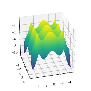
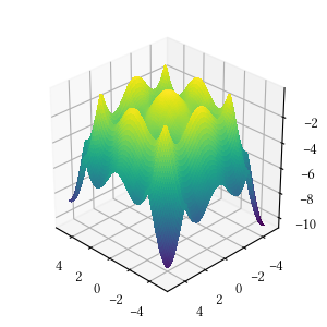
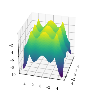
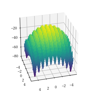
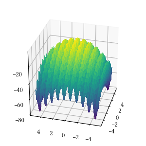
Alpine One
def alpine_one(X):
    return -sum([abs(x * numpy.sin(x) + 0.1 * x) for x in X])
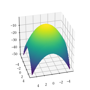
Here is the surface visualization when the optimization dimension is 2.

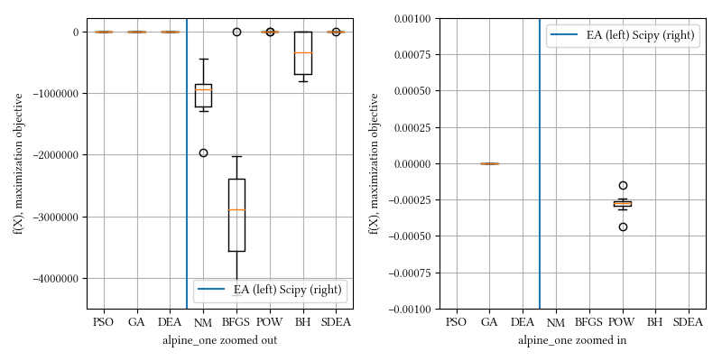
Here is a comparison of optimizer performances when the optimization dimension is 8, and all population-based methods are set to have 100 individuals and 500 iterations with no problem-specific hyper-parameter tuning.
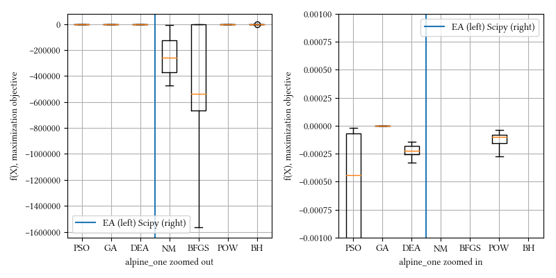
We see BFGS is significantly under-performing than other methods. This is expected. BFGS estimates derivatives from iterations. Since alpine_one is a non-differentiable function, it is not suitable for derivative-aware optimization algorithms, such as BFGS or gradient descent.
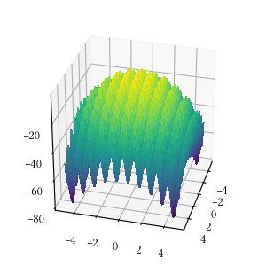
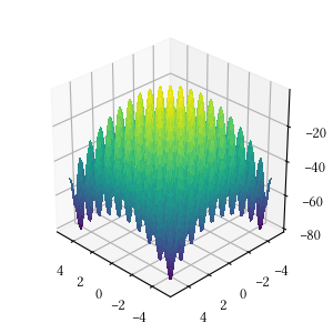
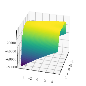
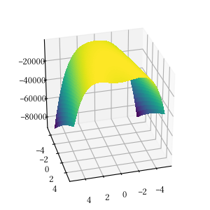
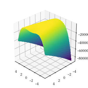
Rastrigin
def rastrigin(X):
    return -(10 * len(X) + sum([(x ** 2 - 10 * np.cos(2 * math.pi * x)) for x in X]))
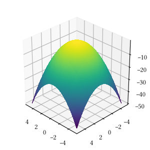
Here is the surface visualization when the optimization dimension is 2.
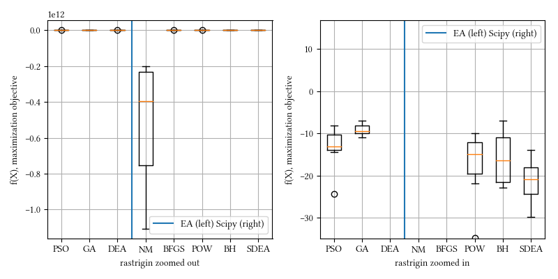
Here is a comparison of optimizer performances when the optimization dimension is 8, and all population-based methods are set to have 100 individuals and 500 iterations with no problem-specific hyper-parameter tuning.
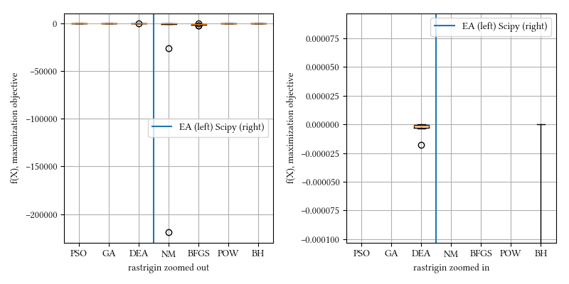
We see here almost all methods, except maybe BFGS, reached a tight and accuracy optima. DEA delivered the best performance. This landscape function is differentiable but have a rough surface.
Rosenbrock
def rosenbrock(X):
    return -sum(
        [100 * (X[i + 1] - X[i] ** 2) ** 2 + (1 - X[i]) ** 2 for i in range(len(X) - 1)]
    )
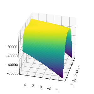
Here is the surface visualization when the optimization dimension is 2.
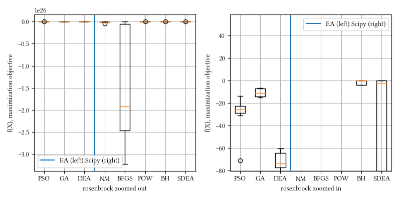
Here is a comparison of optimizer performances when the optimization dimension is 8, and all population-based methods are set to have 100 individuals and 500 iterations with no problem-specific hyper-parameter tuning.
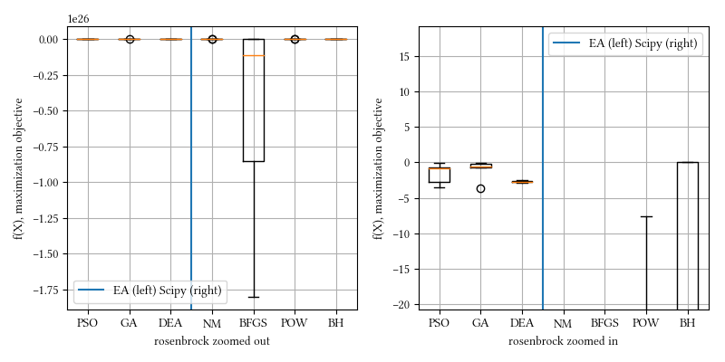
We see here BH and all population-based methods outperform NM, BFGS, and POW. The optimization surface seems relatively straightforward, most non-population based optimizer however, fail. BH has the ingredient of Monte Carlo that creates a somewhat similar behavior as population-base algorithms.
Sphere
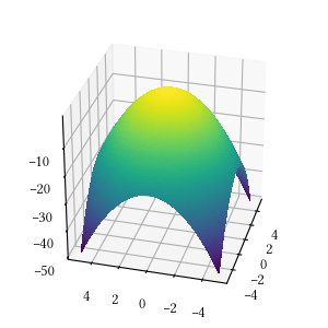
def sphere(X):
    return -sum([x ** 2 for x in X])
Here is the surface visualization when the optimization dimension is 2.

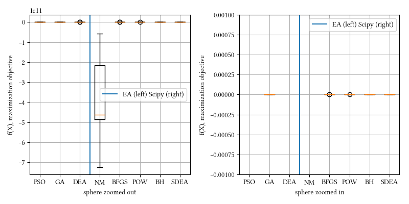
Here is a comparison of optimizer performances when the optimization dimension is 8, and all population-based methods are set to have 100 individuals and 500 iterations with no problem-specific hyper-parameter tuning.
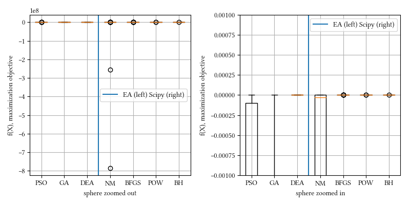
We see here almost all methods reached a tight and accuracy optima, with DEA, BFGS, POW, BH being the best. The optimization is a simple sphere. It should be a straightforward task, and it is most suitable for derivative-aware methods, such as BFGS and gradient descent.
Considerations
We would like to highlight the following considerations when using the evolutionary-optimization package or any black-box derivative-free optimization algorithms.
Parameter space rescaling
Rescaling the parameter space may help the performance significantly for some problems. Our population-based EA algorithms start with an initial set of individuals and follow an algorithmic procedure to explore the parameter space. All encoded solutions are linearly interpolated into interval [0, 1]. This interpolation may not be the absolute best for certain problems. For example, an additional log interpolation can be applied if the parameter space is known to be positive.
Absolute optima
Absolute optima is not always the goal even when the problem formulation is optimization in nature. The most suitable optimization subroutine is not always the one that produces the absolute optima. For example, in a DNN, we optimize a loss function and directly infer edge weights, but we don't care about edge weights themselves. It's likely multiple optima produce the same classification outcome, which is what we care about. In addition, over fitting is a common issue, so it's not advisable to pursue absolute optima. On the other hand, if we optimize a parametrized statistical model where the model parameters are the variable of interest directly, we would want the absolute optima.
Comparison with derivative-aware optimizers
Black-box optimizers are not meant to be compared with derivative-aware optimizers. If we know the analytical form of an objective function, and the derivatives (first, second order) are not crazy to obtain, it's always advisable to take advantage of the derivative information. This, however, is not feasible in many cases, probably the majority engineering scenarios. In addition, black-box optimizers enables a drop-and-go solution that impose no assumption in the objective function as long as we can evaluate it's value given a parameter set, so it's lightweight and could be preferred even at the cost of time or even convergence.
Dimensionality
Black-box optimization algorithms are lightweight but, by nature, they are not capable of dealing with huge parameter dimensions. In cases where function formulation can easily be scaled to have hundreds, thousands, or even more parameters, black-box optimizations would not work. For instance, topic modeling, structure analysis, and DNN, are in this category. Rigorous optimization approaches that make use of the derivatives should be considered, such as back propagation and gradient descent for DNN and quadratic programming in structure analysis. If derivatives are unattainable, then sampling techniques such as MCMC could be a possibility.
Constraints
All test functions used in this discussion are unconstrained. The optimization methods in evolutionary-optimization are created to work with unconstrained problems. This does not mean that these optimizers are incompatible with all constraints. For example, a simple approach to incorporate range constraints is by assigning dis-favorable value, e.g. negative infinity, in the objective function when parameters are out of bounds. This, however, is a relatively dangerous maneuver and often requires extra care during parameter initialization, otherwise optimizers may stuck in a "death" zone and never recover.
Summary
We present evolutionary-optimization, an open-source toolset for derivative-free black-box optimization algorithms. It focuses on evolutionary algorithms, which is a subset of evolutionary computation utilized in the field of artificial intelligence. We can also refer them as generic population-based meta-heuristic optimization algorithms.
Besides the software, this document provides a relatively thorough survey of derivative-free optimization algorithms. Obviously, we do not intend to include all black-box methods. Instead, we aim to cover the best-standing representative in each algorithm family. For example, there exist many other swarm-based algorithms similar to PSO, such as Ant Colony Optimization, Bat Algorithm, and Bee Swarm Optimization. Our implementation of GA is also not the only version. There exist many variations with additional or different genetic manipulations of encoded solutions.
In the experiment section, we see different problems prefer different methods. Non-population based algorithms can be preferable, especially in straightforward optimization problems, such as the high-dimension Sphere function. When the objective surface is rough, such as the Rastrigin function, we see that DEA could be preferable. We observe that a seemingly straightforward objective surface from the Rosenbrock function can pose challenge, and GA outperforms other EA methods. We also had cases [18] where PSO outperforms the rest.
We would like to point out that Scipy provides a version of DEA as well. Here we present another set of experiment that include Scipy's DEA (SDEA). In this experiment, we explore a much higher parameter space dimension, 20 instead of 8 as in the first experiment.
20-param alpine_one:
20-param rastrigin:
20-param rosenbrock:
20-param sphere:
We can see that the best-achieving optimizers are not all the same as in the 8-param experiment. We do not intend to use these results to draw sweeping conclusions about which optimizer is better. No problem-specific tuning was performed on any optimizer. These methods are already proven winners over time. There are many algorithms not included in this discussion, and more are actively been invented. Some are shown better in certain scenarios, but people have learned to be skeptical whenever a claim is made about optimization superiority, unless they are proven repeatedly in other domains, and that is where our selection of algorithms comes from.
In summary, optimization scenarios can be complex and counter intuitive. In reality, we often have little idea of the objective surface, e.g. DNN parameter search, which is thought to be suitable for PSO [19]. It is important to select a suitable method based on the specific problem. Sometimes it even requires hyper-parameter tuning, which can easily be another layer of optimization of its own.
Related Works
J. A. Nelder, R. Mead, A simplex method for function minimization, The Computer Journal 7 (4) (1965) 308-313. doi:10.1093/comjnl/7.4.308.
J. H. Holland, Genetic algorithms, Scientific American 267 (1) (1992) 6672.
D. E. Goldberg, Genetic Algorithms in Search, Optimization and Machine Learning, 1st Edition, Addison-Wesley Longman Publishing Co., Inc., Boston, MA, USA, 1989.
J. E. Baker, Reducing bias and inefficiency in the selection algorithm, in: Proceedings of the Second International Conference on Genetic Algorithms on Genetic algorithms and their application, L. Erlbaum Associates Inc., Hillsdale, NJ, USA, 1987, pp. 14-21.
B. L. Miller, B. L. Miller, D. E. Goldberg, D. E. Goldberg, Genetic algorithms, tournament selection, and the effects of noise, Complex Systems 9 (1995) 193-212.
G. Syswerda, Uniform crossover in genetic algorithms, in: J. D. Schaffer (Ed.), Proceedings of the Third International Conference on Genetic Algorithms, Morgan Kaufmann, 1989, pp. 2-9.
Z. Michalewicz, Genetic algorithms + data structures = evolution programs (1996).
K. Deb, 2001, multiobjetive optimization using evolutionary algorithms (2001).
R. Eberhart, J. Kennedy, A new optimizer using particle swarm theory, in: Proceedings of the Sixth International Symposium on Micro Machine and Human Science, 1995., 1995, pp. 39-43. doi:10.1109/MHS.1995. 494215.
Y. Shi, R. Eberhart, A modified particle swarm optimizer, in: Evolutionary Computation Proceedings, 1998. IEEE World Congress on Computational Intelligence., The 1998 IEEE International Conference on, 1998, pp. 69-73. doi:10.1109/ICEC.1998.699146.
Storn, R. and Price, K., Differential Evolution - a Simple and Efficient Adaptive Scheme for Global Optimization over Continuous Spaces, Technical Report TR-95-012, ICSI, March 1995, ftp.icsi.berkeley.edu. Anyone who is interested in trying Differential Evolution (DE)
S. Paterlini and T. Krink, Differential evolution and particle swarm optimisation in partitional clustering, Comput. Stat. Data Anal., vol. 50, no. 5, pp. 1220-1247, Mar. 2006.
Olson, B., Hashmi, I., Molloy, K. and Shehu, A., 2012. Basin hopping as a general and versatile optimization framework for the characterization of biological macromolecules. Advances in Artificial Intelligence, 2012, p.3.
Vikhar, P. A. "Evolutionary algorithms: A critical review and its future prospects
Cheng, J.Y. and Mailund, T., 2015. Ancestral population genomics using coalescence hidden Markov models and heuristic optimisation algorithms. Computational biology and chemistry, 57, pp.80-92.
Qolomany, B., Maabreh, M., Al-Fuqaha, A., Gupta, A. and Benhaddou, D., 2017, June. Parameters optimization of deep learning models using Particle swarm optimization. In Wireless Communications and Mobile Computing Conference (IWCMC), 2017 13th International (pp. 1285-1290). IEEE.
Powell, M.J., 1964. An efficient method for finding the minimum of a function of several variables without calculating derivatives. The computer journal, 7(2), pp.155-162.
Wales, D J, and Doye J P K, Global Optimization by Basin-Hopping and the Lowest Energy Structures of Lennard-Jones Clusters Containing up to 110 Atoms. Journal of Physical Chemistry A, 1997, 101, 5111.