One of R’s strengths is its powerful formula-based interface to modelling. It saves you the headache of one-hot-encoding categorical variables, manually constructing higher-level interactions, and rewriting models just to add or drop terms. Instead, you just specify the model you want in high-level notation, and R will handle transforming it into the raw numerical model-matrix that’s needed for model-fitting.
Thanks to R’s rich ecosystem of packages, for many situations you’ll find a ready-to-use modelling solution that leverages this formula interface. But there will inevitably be situations where out-of-the-box solutions don’t fit your use-case. When that happens, you’re stuck with something more time-consuming: hand-coding the underlying model-fitting, perhaps using numerical optimization (e.g., stats::optim) or a language like Stan.
We wrote keanu to make tackling situations like these painless and fruitful. It allows you to focus on the core aspects of your models, because it provides tools that handle the busywork of translating abstract model-specifications into the nuts-and-bolts of model-fitting.
Let me introduce the package with a quick example.
An Example
An online retailer is interested in better understanding and predicting the purchasing behavior of a customer segment. This segment consists of customers who visited the website once, didn’t make a purchase, then later returned and made a purchase. The retailer would like to take metrics from that first visit and use them to predict the purchase-amount on the second visit.
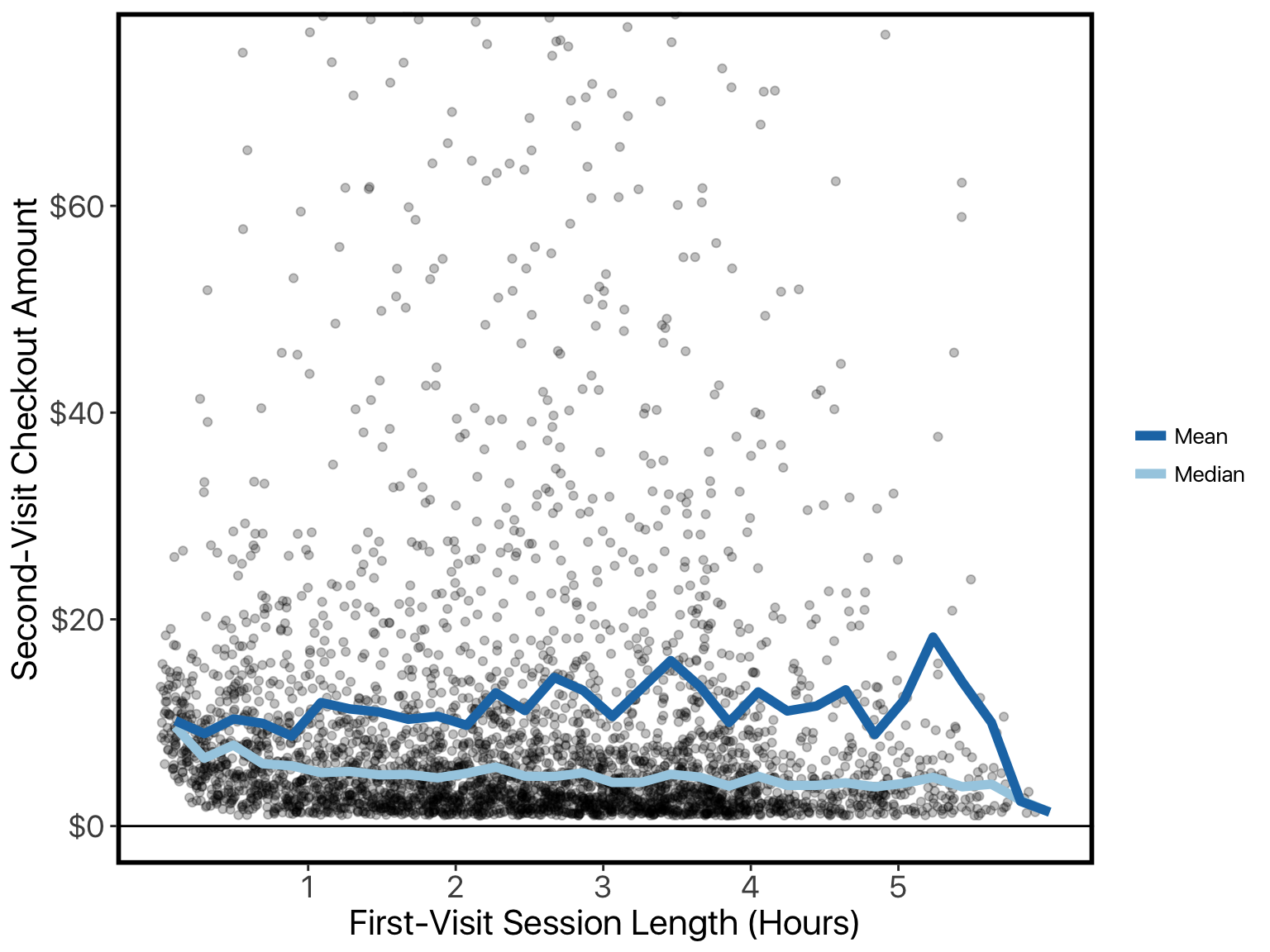
They’re particularly interested in the relationship between first-visit session-length and second-visit purchase-amount:
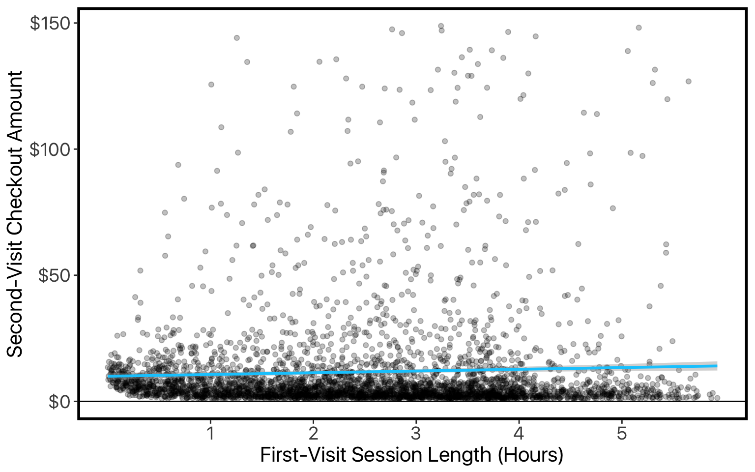
We’d like to better understand these data. We have a handful of predictors, and we’d like to assess how they work together — rather than looking at them in isolation like in the plot above. One simple approach is multiple regression. We’ll try two versions: first on the vanilla data, then after log-transforming the target-variable (since it’s skewed and constrained to be positive).
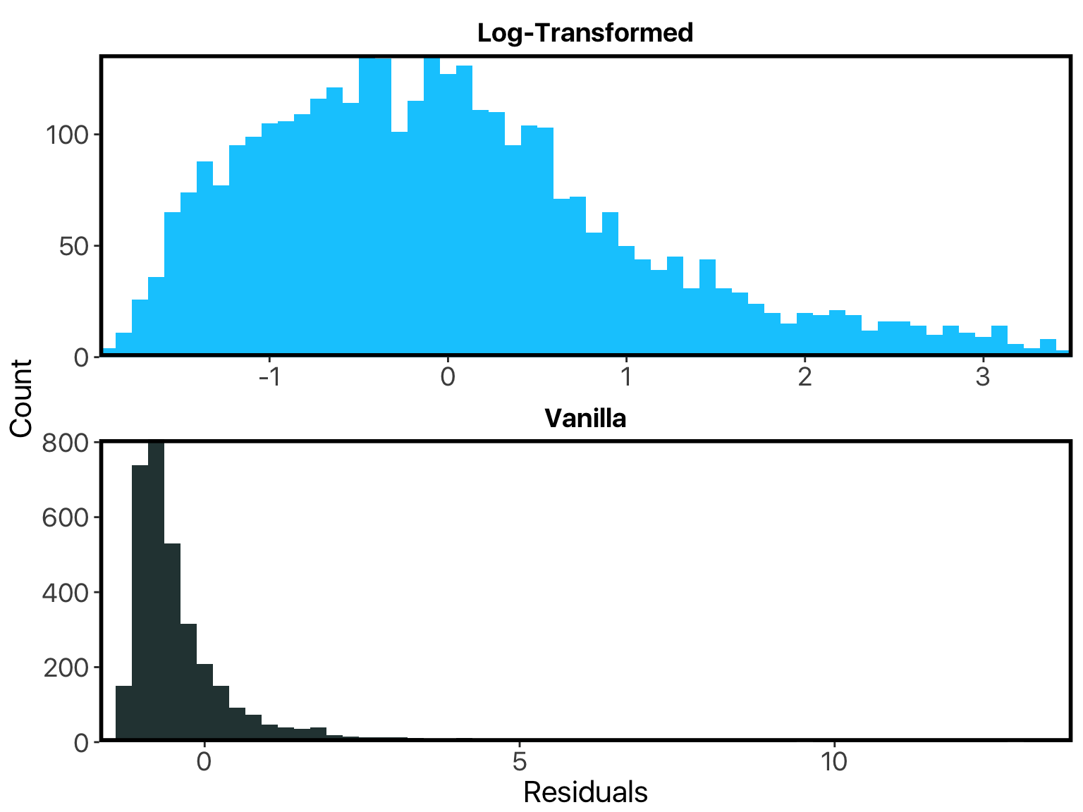
A first glance at the results suggests that the log-transformed model is probably more appropriate: its residuals are more normally-distributed, which is an important assumption in regression models like these. No surprises there.
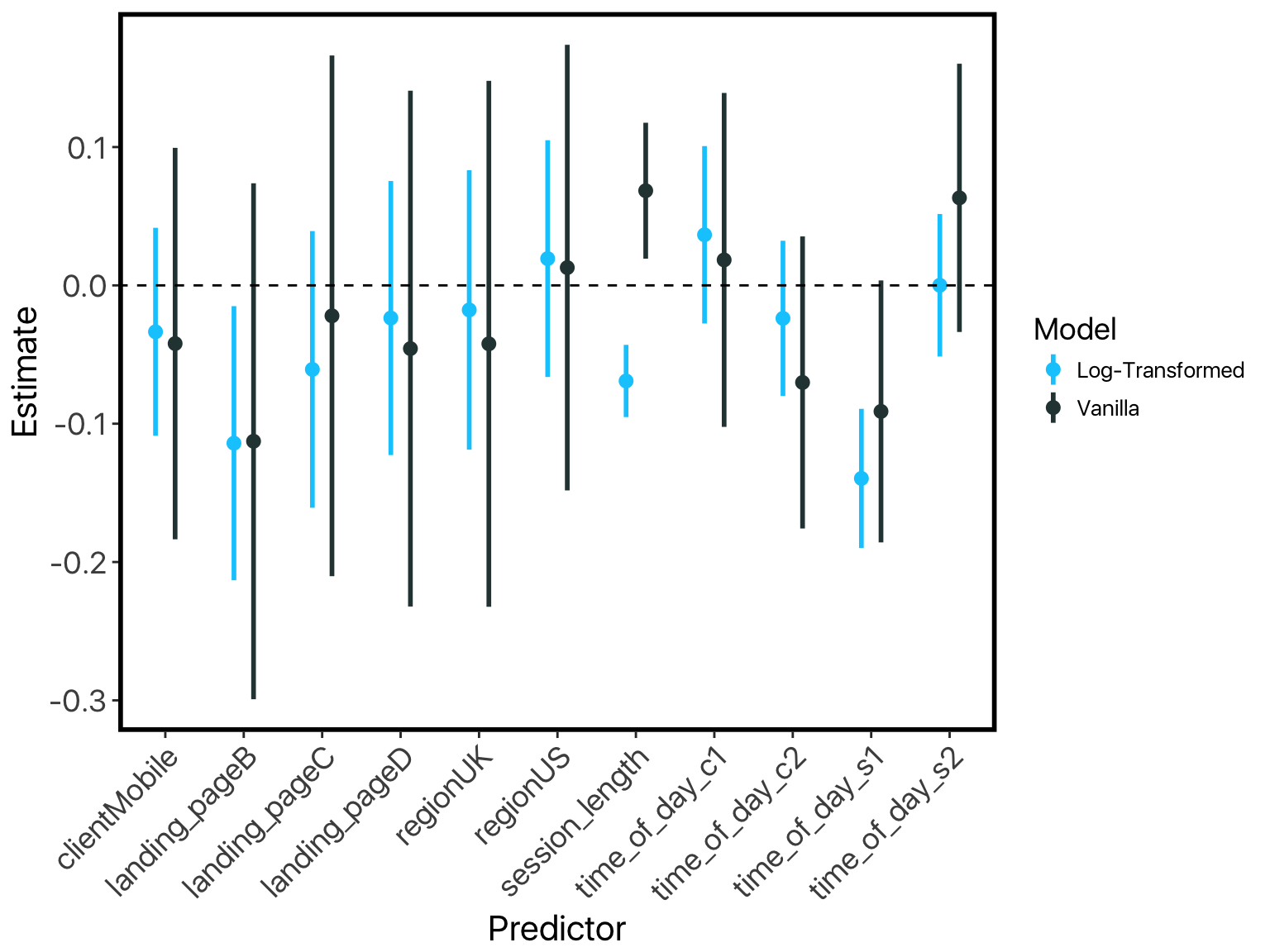
However, if we look closely, something very strange is going on across these two models. Our “session-length” predictor is flipping signs!
We already plotted session-length against checkout amount, where we could clearly see the checkout amount increasing with longer sessions. This matches the vanilla model. The log-transformed model says the opposite. Let’s try re-doing that plot but with log-scaling on our y-axis:
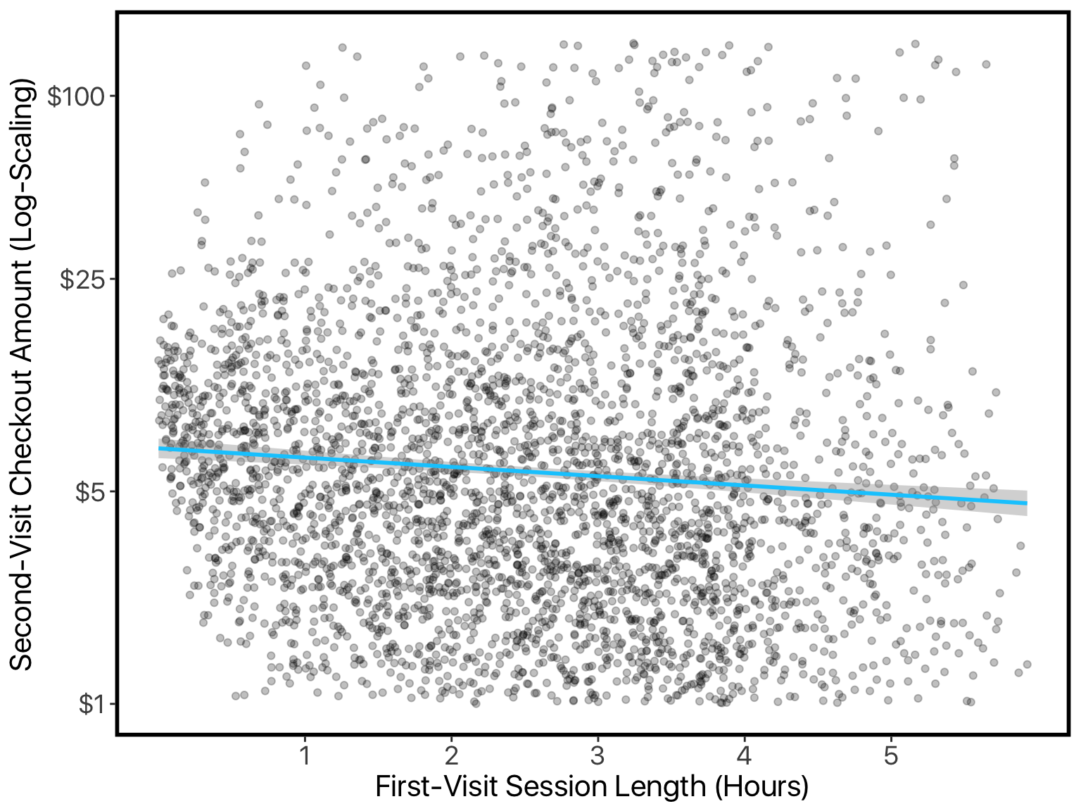
Once we’ve re-scaled the values like this, it looks like longer sessions mean smaller purchases (just like the log-transformed model said).
What is happening here is a conflict between the mean and the median. As session-length goes down, the median checkout-amount goes down. But the variance increases, and checkout amounts are always positive, so this has an asymmetric effect: while the median goes down, the mean goes up.
This is a frustrating situation: two out-of-the-box solutions to modeling our data are giving us conflicting and hard-to-interpret results due to violated model-assumptions. Perhaps we should avoid modeling altogether, using descriptives and visualizations on each predictor separately? Or in the opposite direction, we could spend time coding up a custom model. Neither of these situations are ideal: we’re looking for quick insights in order to drive the more time-consuming, central tasks on the project — we don’t want our kick-off analysis to get bogged down like this.
Keanu in Action
Luckily, keanu offers a better route, by letting us define a custom modeling function like lm within seconds.
Above, we pinned our issue on a conflict between the mean and median. This conflict was due to the fact that, as session-length increases, the median goes down, but the variance goes up. So we just need a model that not only captures the central-tendency of the data, but also its variance.
First, we write out the likelihood function that describes (the error in) our data. The lognormal distribution seems like a good choice, since our data was very close to normally distributed when we log-transformed it.
R provides the density for the lognormal distribution, we’ll just wrap it in a function so that it gives us the log-density by default:
lognormal_loglik_fun <- function(Y, mu, sigma) dlnorm(x = Y, meanlog = mu, sdlog = sigma, log = TRUE)
Next, we just pass this to keanu's modeler_from_loglik. This is a “function factory”: it is a function that produces a function.
lognormal_model <- modeler_from_loglik(loglik_fun = lognormal_loglik_fun)
In this case, the function produced is lognormal_model. It acts a lot like other modeling functions in R, like lm. The biggest difference is that we pass it a list of formulas, instead of a single formula. And instead of just specifying the DV in our formulas, we also specify the parameter of the DV that’s being modeled by that formula.
For example, to model the mu parameter of our checkout_amount_v2 using just session_length, we’d write:
mu(checkout_amount_v2) ~ session_length
For sigma, we’d write something similar. But since the sigma parameter must be greater than zero, we’ll specify a log-link:
sigma(checkout_amount_v2, link = "log") ~ session_length
Now let’s put it all together, using all predictors:
keanu_model <- lognormal_model(

 formulas = list( mu(checkout_amount_v2) ~ .,
 sigma(checkout_amount_v2, link='log') ~ . ),

 data = df_return_segment[c('checkout_amount_v2', predictors)]

)
And… that’s it! Looking at the coefficients (I’ve removed all but the interesting ones to avoid clutter), we see that the model has exactly captured the paradox above. Session-length has a negative coefficient when predicting the mu parameter, but a very large positive coefficient when predicting the sigma parameter:
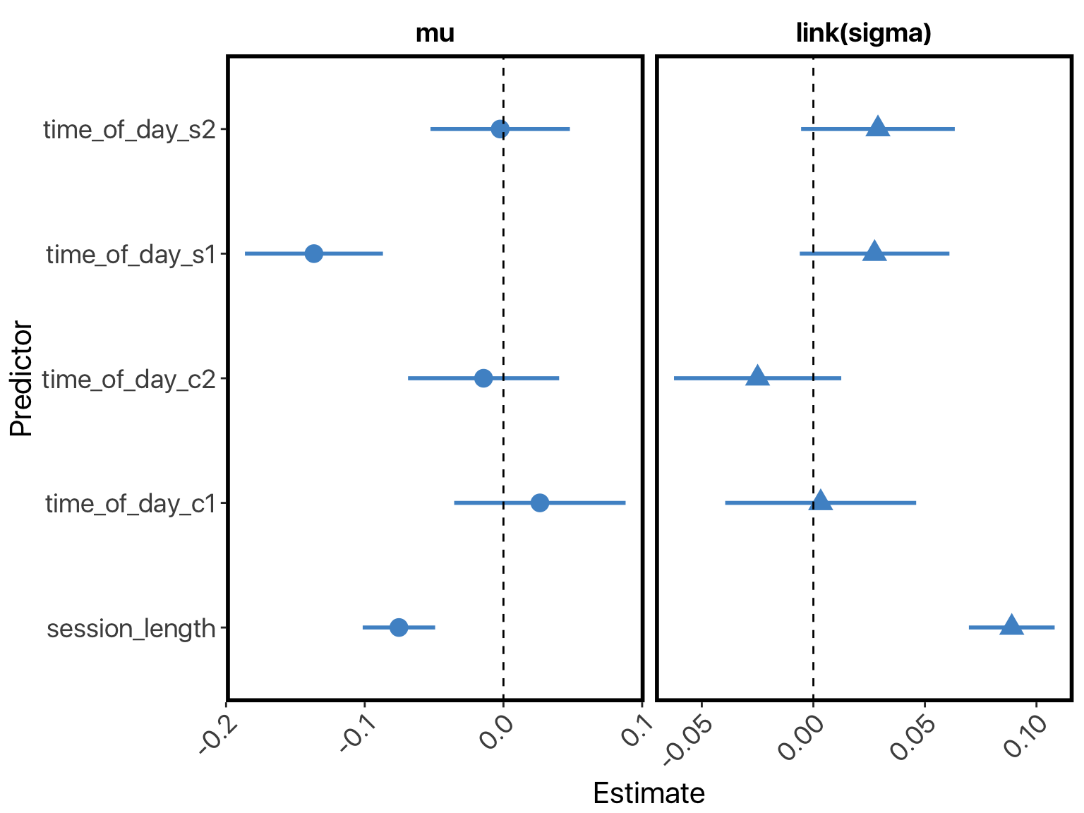
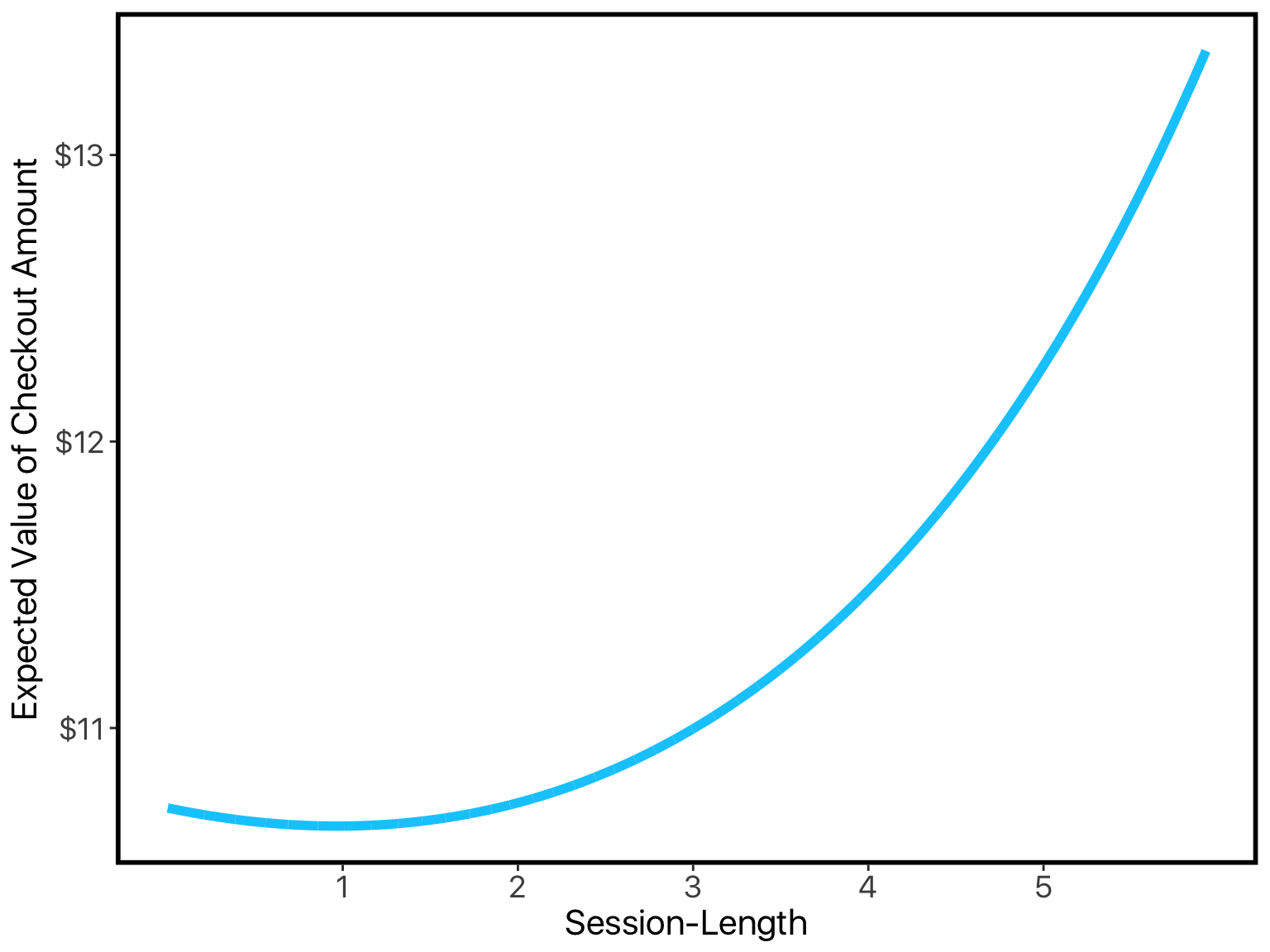
Since the mu parameter of the lognormal distribution corresponds to the median, this explains why the median decreased. Meanwhile, the mean (expected value) of this distribution is given by:
exp(μ+σ22)exp(μ+σ22)
When we plug our coefficients into this, we can see that model correctly captures that the expected-value goes up with longer sessions:
The example here showcases the virtues of keanu nicely. We’ve not only done a better job at building a model that fits our data, but this model also provides more insight than our initial attempts: its coefficient-estimates perfectly capture the paradoxical relationship between session-length and checkout-amount.
So to recap: keanu gives us and fast and easy way of defining modeling functions — all we need to do is provide the likelihood function for our data. These functions let us do quick analyses of data that don’t fit into the mold of out-of-the-box modeling tools in R.
Want to use Keanu in your own work? Check it out on Github.